Quantum mechanics in a Nutshell
Note
The goal of this chapter is to introduce quantum mechanics. There are two aspects to it: the experiment and the theory. Specifically, I will
- describe the phenomenon of atoms/molecules absorb light.
- compare the math of quantum mechanics to the math of stochastic processes.
The precursor of quantum mechanics, known as classical mechanics, is a deterministic theory. Time evolution is described by differential equations such as Newton’s second law
where \(\mathbf F\) is force, \(m\) is mass, \(\mathbf a\) is acceleration, and \(\mathbf x\) is position of an object of interest, say a projectile. Given initial conditions of position and velocity, one can calculate the object’s position at any future time (or even past time).
Although classical mechanics is a successful theory to describe ‘big’ (the physicists’ jargon is macroscopic) objects, its prediction often fails on ‘small’ (microscopic) objects such as molecules and atoms. With the effort of many physicists, quantum mechanics was established in early 20’th century. It is intrinsically a probabilistic theory and is considered bizarre even by the experts. Yet it is a successful theory that seems to have no reported failures on experimental observations.
Overall, its difference from classical mechanics can be summarized as follows
- State space could be finite.
- Superposition of different states is allowed.
- Measurement collapses superposition.
- Dynamics (i.e., transitions between possible states) is probabilistic.
To be concrete, I will use atom as the prototypical quantum object.
absorption spectrum
To illustrate the first difference, let’s revisit Newton’s prism experiment originally recorded in the 17’th century, where a beam of white sunlight passes through a prism and becomes a rainbow of colors, see Fig. 2. From classical optics, we know that light is a wave phenomenon and its color is determined by the wave’s wavelength (or equivalently, its frequency, the speed of light is the same for light of all colors and the light speed is equal to the product of its wavelength and frequency). For example, red light has frequency about 700 nm (460THz), and blue light has frequency about 470 nm (640THz).
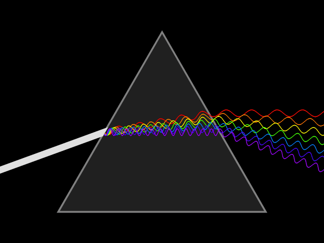
Fig. 2 Newton’s prism experiment.
This simple refraction experiment contains the basic idea of spectroscopy. The plot of light intensity versus light wavelength (or frequency) is called spectrum. An example of the sunlight spectrum is shown in Fig. 3.

Fig. 3 Solar spectrum. The absorption lines are denoted by arrows.
Interestingly, the overall shape of this spectrum reveals the temperature of the Sun. There is a formula relating the light intensity to the light frequency and the temperature of the object, proposed by Max Plank in 1900 and known as Plank’s law. It can also be used to estimate the temperature of a light bulb, or human body. In fact, the derivation of Plank’s law requires quantum mechanics, and it is one of the pioneering work to demonstrate the validity of quantum mechanics. Classical physics gives a non-sensible result in this case, commonly known as the ultraviolet catastrophe of black-body radiation (here black-body simply means a hot object). It predicts that the light intensity approaches infinite at high frequency, for any temperature of the object.
I will not explain Plank’s law here. Instead I would like to draw your attention to some ugly dips in the sunlight spectrum, as denoted by arrows in Fig. 3. These dips are known as Fraunhofer lines. A different view of them is shown in Fig. 4. What happens here is that some of the light is absorbed by various atoms and molecules in the Sun’s atmosphere (actually for stars, it’s called photosphere), causing deviations to Plank’s formula. Interestingly, these absorption lines happens at special frequencies. In fact, they are characteristic of the material. For example, the lines for iron and the lines of oxygen molecules look nothing like each other. Thus by looking at these lines, we can deduce the composition of the Sun and even their abundance.

Fig. 4 Solar spectrum with Fraunhofer lines.
But what does it mean that iron (or any other atoms or molecules) has multiple absorption lines? One hypothesis could be that iron atom has multiple states and each state corresponds to one particular line. This is actually not too far from the full story. The more complete explanation is as follows
- Each dark line means the absence of light with specific wavelength (or frequency);
- That specific light carries a specific amount of energy;
- The iron atom has two states whose energy difference equals to that specific light’s energy, and it is able to absorb the light and jump from the low energy state to the high energy state.
The first point merely states experimental observation. The latter two points are both alien to the 19’th century physicists. Nowadays they are known to the general public. For example, sunscreens contain special molecules that absorb ultraviolet (UV) (high frequency/short wavelength) light. If the UV light is not blocked by sunscreen, molecules in our skin may absorb them and become something else.
One confusing subtlety of light can be summarized in this question: does a dim UV light carry more energy or less energy than a bright red (red is long wavelength/low frequency) light? One way to think about this is to imagine light as a flux of flying balls (the balls are known as photons). Two factors contributes to the light source’s intensity, or brightness, or illuminance or radiance as coined by the pros:
- the number of balls hit a unit area in a unit time, i.e., the flux
- the energy carried by each ball: a purple ball has more energy than a red ball
Thus it is possible that a dim UV light (small flux) bombast one’s skin (of a fixed area and in a fixed time span) with less energy than a bright red light. However, red light is much less likely to be absorbed by the skin thus it doesn’t cause as much harm as a dimmer UV light even though it carries more energy.
Now let me illustrate why it’s weird for an atom (or molecule) to be in a finite number of states. By that time, physicists already knew that atoms are made of nucleus with positive charge and electrons with negative charge. If one makes the analogy that nucleus is the Sun, an electron is a planet, and the attractive force between positive and negative charges plays the role of gravitational attraction, it is unclear why only a finite number of stable orbits exist. Note that in the Sun-and-planet case, there are infinite stable orbits, although only a few of them are occupied. If we launch a new satellite, we pre-calculate the stable orbit so that it doesn’t hit into other things. And if the satellite’s speed increase a little bit, it will be in a slightly different orbit.
Again the full explanation require quantum mechanics.
See also
Spectroscopy is likely the most important experimental technique in modern science.
I don’t known any convincing explanation about why microscopic objects often assume discrete states. For example, these atomic states are not energy minimums of some cost function. However, the evidence of them are quite strong, thus a successful theory has to incorporate them. As a result, quantum theory is bizarre.
All models are wrong; some are useful. — George E. P. Box
analogy of coin tossing
Quantum mechanics is intrinsically a probabilistic theory, that is, if one repeats an experimental procedure in an idealized situation (no human mistake, no machine error, no noise) with a measurement at the end, the measurement results could still differ from different trials. At a superficial level, it is similar to probability theory where some information is not available.
The simplest quantum system has two states and the classical analogy is a coin with two sides. A coin toss has two outcomes: head and tail, and is represented by Bernoulli distribution:
Each coin toss has two outcomes and their probabilities can be described by a two-component vector \(\mathbf p\). For example, fair coins have
Given such probability vectors, we can easily describe the tossing of the same coin many times, or more generally, the tossing of many coins with different biases. Take two coins for example, the outcome probability is given by the tensor product of the individual probability vectors, i.e.,
With \(n\) different coins, there are \(2^n\) possible states. However, the probabilities can be calculated from \(2n\) numbers. This is the product rule of probability since we assume the coin tosses are independent events.
To make the situation more complicated, there are two ways to go:
- make the coin tosses dependent events: maybe they hit each other as they are tossed (instead of being tossed one by one)
- make the probability distribution time-dependent: maybe they are being deformed as they are tossed
The first complication breaks the product rule and we have to assign one probability to each outcome. In the two-coin example,
and no decomposition is possible anymore.
The second complication adds dynamics to the probabilities distributions. The simplest description one can give may be the Kolmogorov equation:
\(\frac{d}{dt}\mathbf{p}(t)=R\mathbf{p}(t)\)
where \(R\) is a transition rate matrix.
For simplicity, let’s assume that \(R\) is time-independent. Then we have a formal solution
\(\mathbf p(t) = e^{Rt}\mathbf p(0).\)
‘quantum’ coin tossing
If we magically force a coin to obey quantum mechanics, some of its behavior would appear identical to the classical coin. For example, if we ‘toss’ the quantum coin, there will still be only two outcomes, head or tail, just like the classical coin. This ‘quantum’ coin tossing is called von Neumann measurement in quantum mechanics, which is the equivalent of drawing one sample from a probability distribution. If we toss many quantum coins with identical states, the outcomes of head or tail also follow Bernoulli distribution.
Before we proceed to the difference between quantum coin and classical coin, let’s first prepare ourselves with the notation for describe quantum states, i.e., the Dirac notation.
Dirac notation
The state of the quantum coin is described by a 2D complex vector
where \(c_H, c_T\in \mathbb{C}\) and they are called probability amplitudes. Here \(\left|H\right>\) and \(\left|T\right>\) are called basis states, and \(\left|\psi\right>\) is known as the wave function.
If we tossing the quantum coin many times, the probabilities to get head or tail are given by \(\|c_H\|^2\) and \(\|c_T\|^2\). And we have the normalization \(\|c_H\|^2 + \|c_T\|^2 = 1\).
Here the half bracket notation is called the Dirac notation. In this example, they correspond to 2D vectors:
These states with right bracket are called ket(s). Paul Dirac also defined the complex conjugate of these vectors
Such states with left bracket are called bra(s). And overall Dirac notation is also called bra-ket notation. With this notation, probability normalization can be written succinctly as
One could argue that it is not really more convenient than \(\mathbf c^\dagger \mathbf c=1\), which I agree. I think its power is slightly more evident when there are uncountable infinite possible states. In the end, it is just a notation that physicists are used to.
For multiple quantum coins, their state vector is also tensor product of the individual ones. Take the two coin case for example,
Again, if the two quantum coins are somehow coupled together, such decomposition is not possible,
If we go back to the absorption spectrum example, \(\left|\psi_1\right> \otimes \left|\psi_2\right>\) represent two atoms, each of which has two internal states. Thus at most two absorption lines can be observed. On the other hand, the state of coupled coins could also model an atom with four internal states. In that case at most \(C(4, 2)=6\) absorption lines can be observed.
Now if we identify \(p_i = c_i^*c_i\), then it appears the quantum case maps to the classical case exactly. And it seems unnecessary to use complex numbers instead of real numbers. This superficial similarity will be examined more closely in the following sections.
superposition principle and quantum measurement
Before going to the time evolution of quantum mechanics, let me first reveal the differences between classical probability theory and quantum mechanics in static situations.
The analogy between probability theory and quantum mechanics is summarized in Table 2. Both the superposition principle and von Neumann measurement differ from their probabilistic counterpart at fundamental level.
| probability theory | quantum mechanics |
|---|---|
| multiple possible states | superposition principle |
| drawing sample from a distribution | von Neumann measurement |
The peculiarities of the superposition principle are
- Different states can be linearly superimposed.
- The coefficients of such superposition are complex numbers.
In probability theory, statistics, or ensemble average, is calculated as
where \(f_i\) is some numerical value assigned to the state. For example, we can assign \(f\) to \(1\) for head, and \(-1\) for tail.
In the same spirit, a quantum ensemble average could take the same form
The acute reader may find Eq. (3) puzzling. In the coin example, \(\left|\psi\right>\) is a 2-by-1 vector, thus it appears that \(f\) should be a 2-by-2 matrix. This is indeed true. Since I use capital letters to denote matrix, the quantum ensemble average should take the form of
where \(F_{ii}\) may correspond to \(f_i\). But what is the meaning of the off diagonal terms \(F_{ij}\)? Actually they don’t have classical correspondence in probability theory. They are put in there to model wave interference, which takes care of the discrepancy to the predictions of classical mechanics. It is an intrinsic nature of quantum mechanics (note that quantum mechanics is also known as wave mechanics and the state vector is known as wave function).
These off-diagonal terms together with the \(c_i\) being complex numbers provide more degrees of freedom to explain experimental observations that deviate from classical expectations in Eq. (2). Note that I didn’t explain why the quantum ensemble takes the form of Eq. (4). In fact, I don’t know any high-level plausible ideas why it should be, except that the formalism works.
The value of the off-diagonal terms is not completely arbitrary. There is controversy of whether complex numbers are physical (i.e., whether they can be measured from an experiment) or they are only mental constructions to simplify notations (I tend to take the latter view). For the sake of argument, let’s assume that measurement can only yield real numbers. This requirement puts on extra constraint on the form of \(F\) since \(\left<\psi\right|F \left|\psi\right>\) has to be real for any vector \(\left|\psi\right>\). The qualified class is called Hermitian matrix.
As a summary, the main difference introduced in the superposition principle is the off-diagonal terms in the observation, which models interference.
Measurement in quantum mechanics is radically different: after a quantum coin toss, the coin’s probability amplitude (thus probability distribution) changes.
Suppose the coin is in state of Eq. (1) before the measurement. After the measurement, its state changes to either \(\left|H\right>\) or \(\left|T\right>\) with the corresponding probability. Any subsequent measurement gives deterministic result. In other words, tossing the same quantum coin multiple times doesn’t work because the quantum coin is not the same after a toss (unless it’s in one of the basis states to start with). This phenomenon is known as wave function collapse. In our analogy, we could also call it probability distribution collapse.
On the other hand, if we toss an ensemble of quantum coins with identical state (i.e., probability amplitude or probability distribution), we will observe the same head and tail counts as in probability theory. In general, if we want to observe some physical quantity as in Eq. (4), an ensemble of quantum states is needed. This ensemble can be generated either by repeatedly preparing and measuring the same quantum object, or preparing the same state for many quantum objects and measuring them.
dynamics
There are two
- von Neumann measurement
- time evolution
the mathematics to describe the coin will change quite dramatically.
Similar to the classical case, in the case when \(H\) is time independent, Schrodinger equation has explicit solution
In general, the solution can be very complicated when the Hamiltonian is time dependent.
where \(U(t)\) absorbs all the complications in it and is simply called the time evolution.
Probability conservation \(\mathbf c^\dagger \mathbf c=1\) puts on requirement on the time evolution matrix
This type of matrices are called unitary matrix.
The simplest time-dependent Hamiltonian may be one that is piecewise constant. Suppose during time interval \(\Delta t_i\), the Hamiltonian is \(H_i\), then we have
This is a common scheme to build time evolution out of a handful Hamiltonians. Here the control variables are the ordering of the available Hamiltonians and their time intervals.
A side-by-side comparison of quantum mechanics and stochastic processes is shown in Table 3.
| stochastic process | quantum mechanics | |
|---|---|---|
| state vector | probabilities \(\mathbf p\) | probability amplitudes \(\mathbf c\) |
| normailization | \(\|\mathbf p\|_1 = 1\) | \(\mathbf c^\dagger \mathbf c =1\) |
| dynamics |
|
|
| solution | \(\mathbf p(t) = e^{Rt}\mathbf p(0)\) | \(\mathbf c(t)=e^{-iHt}\mathbf c(0)\) |
See also
Here I only presented the equations and notations used in quantum mechanics, but didn’t explain how they come into being. The